2 Chapter 2 exercises
Compute \(\pi + \text{e}\), where \(\pi = 3.1415927 \times 10^0\) and \(\text{e} = 2.7182818 \times 10^0\), using floating point addition in base 10, working to five decimal places.
Solution
As \(\pi\) and \(\text{e}\) have a common exponent, we sum their mantissas, i.e. \[\begin{align*} \pi + \text{e} &= (3.14159 \times 10^0) + (2.71828 \times 10^0)\\ &= 5.85987 \times 10^0 \end{align*}\]
Now compute \(10^6\pi + \text{e}\), using floating point addition in base 10, now working to seven decimal places.
Solution
We first need to put the numbers on a common exponent, which is that of \(10^6 \pi\). \[\begin{align*} 10^6 \pi &= 3.1415927 \times 10^6\\ \text{e} & = 2.7182818 \times 10^0 = 0.0000027 \times 10^6. \end{align*}\] Then summing their mantissas gives \[\begin{align*} 10^6 \pi + \text{e} &= (3.1415927 \times 10^6) + (2.7182818 \times 10^0)\\ &= (3.1415927 \times 10^6) + (0.0000027 \times 10^6)\\ &= (3.1415927 + 0.0000027) \times 10^6\\ &= 3.1415954 \times 10^6. \end{align*}\]
What would happen if we computed \(10^6\pi + \text{e}\) using a base 10 floating point representation, but only worked with five decimal places?
Solution
If we put \(2.7182818 \times 10^0\) onto the exponent \(10^6\) we get \(0.00000 \times 10^6\) to five decimal places, and so \(\text{e}\) becomes negligible alongside \(10^6 \pi\) if we only work to five decimal places.
Write \(2\pi\) in binary form using single- and double precision arithmetic. [Hint: I recommend you consider the binary forms for \(\pi\) given in the lecture notes, and you might also use
bit2decimal()from the lecture notes to check your answer.]
Solution
The key here is to note that we want to calculate \(\pi \times 2\). As we have a number in the form \(S \times (1 + F) \times 2^{E - e}\), then we just need to raise \(E\) by one. For both single- and double-precision, this corresponds to changing the last zero in the 0s and 1s for the \(E\) term to a one.
bit2decimal <- function(x, e, dp = 20) {
# function to convert bits to decimal form
# x: the bits as a character string, with appropriate spaces
# e: the excess
# dp: the decimal places to report the answer to
bl <- strsplit(x, ' ')[[1]] # split x into S, E and F components by spaces
# and then into a list of three character vectors, each element one bit
bl <- lapply(bl, function(z) as.integer(strsplit(z, '')[[1]]))
names(bl) <- c('S', 'E', 'F') # give names, to simplify next few lines
S <- (-1)^bl$S # calculate sign, S
E <- sum(bl$E * 2^c((length(bl$E) - 1):0)) # ditto for exponent, E
F <- sum(bl$F * 2^(-c(1:length(bl$F)))) # and ditto to fraction, F
z <- S * 2^(E - e) * (1 + F) # calculate z
out <- format(z, nsmall = dp) # use format() for specific dp
# add (S, E, F) as attributes, for reference
attr(out, '(S,E,F)') <- c(S = S, E = E, F = F)
out
}
bit2decimal('0 10000001 10010010000111111011011', 127)
## [1] "6.28318548202514648438" ## attr(,"(S,E,F)") ## S E F ## 1.0000000 129.0000000 0.5707964## [1] "6.28318530717958623200" ## attr(,"(S,E,F)") ## S E F ## 1.0000000 1025.0000000 0.5707963Find the calculation error in
Rof \(b - a\) where \(a = 10^{16}\) and \(b = 10^{16} + \exp(0.5)\).
Create the following: The row vector \[ \mathbf{a} = (2, 4, 6), \] the \(2 \times 3\) matrix \[ \mathbf{B} = \left(\begin{array}{ccc} 6 & 5 & 4\\ 3 & 2 & 1\end{array}\right) \] and a list with first element \(\mathbf{a}\) and second element \(\mathbf{B}\), and an arbitrary (i.e. with whatever values you like) \(5 \times 3 \times 2\) array with a
'name'attribute that is'array1'. \(~\)
For each of the above, consider whether your code could be simpler.
Solution
a <- t(c(2, 4, 6))
B <- matrix(6:1, 2, byrow = TRUE)
l <- list(a, B)
arr <- array(rnorm(30), c(5, 3, 2))
attr(arr, 'name') <- 'array1'
arr
## , , 1 ## ## [,1] [,2] [,3] ## [1,] 0.09189745 -1.1100867 1.0556685 ## [2,] 0.48984616 1.0004907 -1.1530448 ## [3,] 0.62202232 1.0721109 -2.0391218 ## [4,] -1.13829291 -0.7489970 1.4121921 ## [5,] -0.44677627 0.5844577 0.4677163 ## ## , , 2 ## ## [,1] [,2] [,3] ## [1,] 0.5892771 1.53977989 -0.3380553 ## [2,] 0.7235191 -0.26054324 1.1023774 ## [3,] -0.5613542 -0.98918746 2.6263768 ## [4,] 0.6259059 -0.09356743 1.0588086 ## [5,] 1.2621820 -1.23706785 0.8464913 ## ## attr(,"name") ## [1] "array1"Produce a \(3 \times 4 \times 4 \times 2\)
arraycontaining Uniform(0, 1) random variates and compute the mean over its second and third margins usingapply(..., ..., means)androwMeans()orcolMeans().
Solution
arr <- array(NA, c(3, 4, 4, 2))
arr[] <- runif(prod(dim(arr))) # saves names to get the number right
apply(arr, 2:3, mean)
## [,1] [,2] [,3] [,4] ## [1,] 0.3277448 0.3154984 0.4548109 0.3079770 ## [2,] 0.4490244 0.5035501 0.4321672 0.5970750 ## [3,] 0.4240671 0.5412790 0.6083608 0.3464060 ## [4,] 0.4118282 0.6029751 0.5059753 0.4539781## [,1] [,2] [,3] [,4] ## [1,] 0.3277448 0.3154984 0.4548109 0.3079770 ## [2,] 0.4490244 0.5035501 0.4321672 0.5970750 ## [3,] 0.4240671 0.5412790 0.6083608 0.3464060 ## [4,] 0.4118282 0.6029751 0.5059753 0.4539781## [,1] [,2] [,3] [,4] ## [1,] 0.3277448 0.3154984 0.4548109 0.3079770 ## [2,] 0.4490244 0.5035501 0.4321672 0.5970750 ## [3,] 0.4240671 0.5412790 0.6083608 0.3464060 ## [4,] 0.4118282 0.6029751 0.5059753 0.4539781Create a 3-element
listof vectors comprising Uniform(0, 1) variates of length 3, 5 and 7, respectively.
Create another list in which the vectors above are sorted into descending order.
Then create a vector comprising the minimum of each vector in the list, and another stating which element is the minimum. [Hint: for the latter you may want to consult the ‘See Also’ part of the
min()function’s help file.]
Solution
## [1] 0.19104777 0.23805009 0.04880771## [1] 1 5 3
Use a
for()loop to produce the following. [Hint: the functionpaste()might be useful.]## [1] "iteration 1" ## [1] "iteration 2" ## [1] "iteration 3" ## [1] "iteration 4" ## [1] "iteration 5" ## [1] "iteration 6" ## [1] "iteration 7" ## [1] "iteration 8" ## [1] "iteration 9" ## [1] "iteration 10"
Solution
## [1] "iteration 1" ## [1] "iteration 2" ## [1] "iteration 3" ## [1] "iteration 4" ## [1] "iteration 5" ## [1] "iteration 6" ## [1] "iteration 7" ## [1] "iteration 8" ## [1] "iteration 9" ## [1] "iteration 10"Consider the following two infinite series that represent \(\pi\).\[\begin{align*} \pi &= 4 \left[1 - \frac{1}{3} + \frac{1}{5} - \frac{1}{7} + \frac{1}{9} - \frac{1}{11} + \frac{1}{13} -\cdots\right]\\ \pi &= 3 + \frac{4}{2 \times 3 \times 4} - \frac{4}{4 \times 5 \times 6} + \frac{4}{6 \times 7 \times 8} - \frac{4}{8 \times 9 \times 10} + \cdots \end{align*}\] Use a
while()loop to find which converges topiinRto within \(\epsilon_m^{1/3}\) using the fewest terms, where \(\epsilon_m\) isR’s machine tolerance.
Solution
Here’s the first approximation…
quarter_pi <- 1
terms1 <- 1
denom <- 3
multiplier <- -1
my_pi <- 4 * quarter_pi
while(abs(my_pi - pi) > .Machine$double.eps^(1/3)) {
  terms1 <- terms1 + 1
  quarter_pi <- quarter_pi + multiplier / denom
  my_pi <- 4 * quarter_pi
  denom <- denom + 2
  multiplier <- -1 * multiplier
}
terms1
## [1] 165141…and here’s the second approximation…
my_pi <- 3
terms2 <- 2
denoms <- c(2, 3, 4)
multiplier <- 1
while(abs(my_pi - pi) > .Machine$double.eps^(1/3)) {
  my_pi <- my_pi + multiplier * 4 / prod(denoms)
  denoms <- denoms + 2
  multiplier <- -1 * multiplier
  terms2 <- terms2 + 1
}
terms2
## [1] 36Write a function based on a
for()loop to calculate the cumulative sum of a vector, \(\bf y\), i.e. so that its \(i\)th value, \(y_i\) say, is \[y_i = \sum_{j = 1}^i x_j.\]
Solution
Either of the following two functions are options (although others exist).
my_cumsum <- function(x) {
# function 1 to calculate cumulative sum of a vector
# x is a vector
# returns a vector of length length(x)
out <- numeric(length(x))
for (i in 1:length(x)) {
  out[i] <- sum(x[1:i])
}
out
}

my_cumsum2 <- function(x) {
# function 2 to calculate cumulative sum of a vector
# x is a vector
# returns a vector of length length(x)
out <- x
for (i in 2:length(x)) {
  out[i] <- out[i] + out[i - 1]
}
out
}
We see that both perform the same calculation.
## [1] 0.9865736 1.7893478 1.8637196 2.7207006 3.5074895 4.2404882 4.2755239 5.0113224 5.5099278 5.6815535## [1] 0.9865736 1.7893478 1.8637196 2.7207006 3.5074895 4.2404882 4.2755239 5.0113224 5.5099278 5.6815535## [1] 0.9865736 1.7893478 1.8637196 2.7207006 3.5074895 4.2404882 4.2755239 5.0113224 5.5099278 5.6815535Then benchmark its execution time against
R’s vectorised functioncumsum()for summing 1000 iid \(Uniform[0, 1]\) random variables.
Solution
## Unit: nanoseconds
To start a board game, a player must throw three sixes using a conventional die. Write a function to simulate this, which returns the total number of throws that the player has taken.
Solution
Then use 1000 simulations to empirically estimate the distribution of the number of throws needed.
Solution
## samp1
##  3  4  5  6  7  8  9 10 11 12 13 14 15 16 17 18 19 20 21 22 23 24 25 26 27 28 29 30 31 32 33 34 35 36 37 38 39 40 42 43 44 45 46 48 49 51 52 53 54 55 57 60 61 64 72
##  2 17 23 31 29 44 40 49 51 50 46 44 48 56 43 33 40 41 23 32 31 14 20 23 15 22 13 14 10  7  9  5  7  9  6  5  5  2  9  4  6  4  4  1  1  2  1  2  1  1  1  1  1  1  1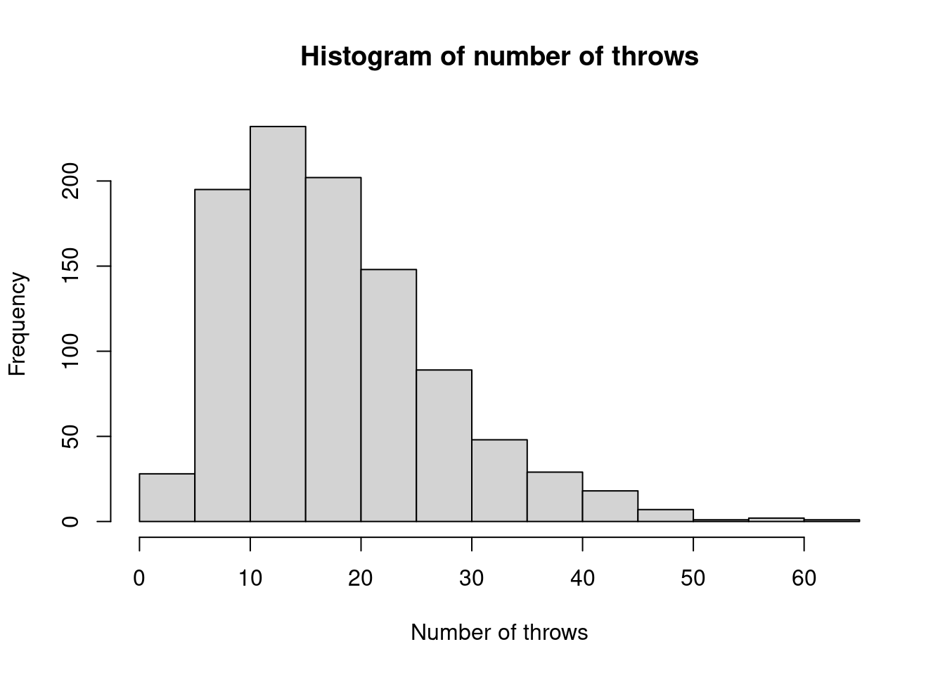
Figure 2.1: Histogram of empirical distribution of number of throws for starting method 1.
I think you’ll agree that this would be a rather dull board game! It is therefore proposed that a player should instead throw two consecutive sixes. Write a function to simulate this new criterion, and estimate its distribution empirically.
Solution
sixes2 <- function() {
# function to simulate number of throws needed
# for two consecutive sixes
# n is an integer
# returns total number of throws taken
out <- sample(1:6, 2, replace = TRUE)
cond <- TRUE
while(cond) {
  if (sum(out[1:(length(out) - 1)] + out[2:length(out)] == 12) > 0) {
    cond <- FALSE
  } else {
    out <- c(out, sample(1:6, 1))
  }
}
return(length(out))
}
sixes2()
## [1] 143Then use 1000 simulations to empirically estimate the distribution of the number of throws needed.
Solution
## samp2
##   2   3   4   5   6   7   8   9  10  11  12  13  14  15  16  17  18  19  20  21  22  23  24  25  26  27  28  29  30  31  32  33  34  35  36  37  38  39  40  41  42  43  44
##  27  21  17  21  15  35  23  23  20  25  17  16  16  13  18   9  20  18  18  18  14   9  17  14   9  14  11  20   9   8  10   6  11   7   5  12  12   7  10   5   7  13  10
##  45  46  47  48  49  50  51  52  53  54  55  56  57  58  59  60  61  62  63  64  65  66  67  68  69  70  71  72  73  74  75  76  77  78  79  80  81  82  83  84  85  86  87
##  13  12   8  13   5   9   5   3   9   5   7  10   7   7   3   5   7   4   5   4   3   4   5   4   5   3   5   2   9   1   5   4   8   4   2   3   6   2   9   2   3   4   1
##  88  89  90  91  92  93  94  95  96  97  98  99 100 101 102 103 104 105 107 108 109 110 112 113 114 115 116 117 119 120 121 122 123 124 126 128 129 130 131 133 136 137 138
##   2   4   1   3   2   1   4   5   5   2   3   3   1   7   4   3   4   2   3   1   4   1   2   2   1   1   3   1   1   1   1   3   2   2   1   1   1   2   2   3   1   2   1
## 139 141 142 143 144 145 148 152 154 156 158 159 161 163 168 170 173 177 182 190 191 199 211 214 216 217 222 225 241 277 291
##   1   2   2   2   1   1   2   2   1   1   1   1   1   1   1   1   1   1   1   1   1   1   1   1   1   1   1   1   1   1   1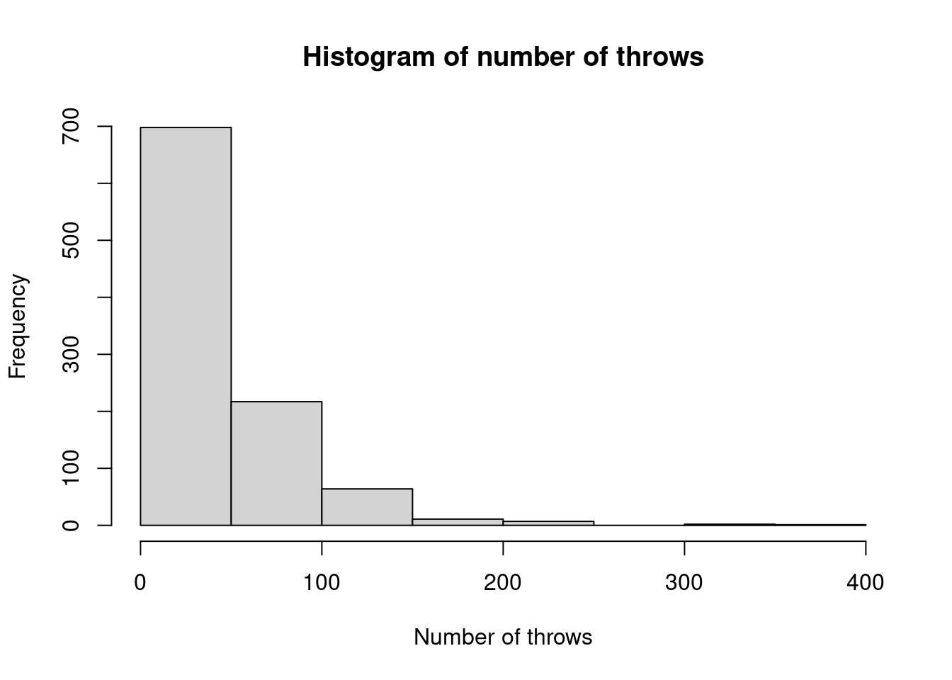
Figure 2.2: Histogram of empirical distribution of number of throws for starting method 2.
By comparing sample mean starting numbers of throws, which starting criterion should get a player into the game quickest?
Solution
## [1] -25.433So the second approach, by comparing means, takes more throws before the game can begin.
Consider the following two functions for calculating \[d_i = x_{i + 1} - x_i, \hspace{2cm} i = 1, \ldots, n - 1\] where \({\bf x}' = (x_1, \ldots, x_n)\).
diff1 <- function(x) {
# function to calculate differences of a vector
# based on a for loop
# x is a vector
# returns a vector of length (length(x) - 1)
out <- numeric(length(x) - 1)
for (i in 1:(length(x) - 1)) {
  out[i] <- x[i + 1] - x[i]
}
out
}
diff2 <- function(x) { # function to calculate differences of a vector # based on vectorisation # x is a vector # returns a vector of length (length(x) - 1) id <- 1:(length(x) - 1) x[id + 1] - x[id] }The first,
diff1()uses a straightforwardfor()loop to calculate \(d_i\), for \(i = 1, \ldots, n - 1\), whereasdiff2()could be seen to be a vectorised alternative. Benchmark the two for a vector of \(n = 1000\) iid \(N(0, 1)\) random variates by comparing the median difference in execution time.
Solution
## Unit: microsecondsThe following function assesses whether all elements is a logical vector are
TRUE.all2 <- function(x) { # function to calculate whether all elements are TRUE # returns a scalar # x is a logical vector sum(x) == length(x) }Calculate the following and benchmark
all2()againstR’s built-in functionall(), which does the same.
Solution
## [1] TRUE## [1] TRUE## Unit: microsecondsWe see that both take a similar amount of time.
Now swap the first element of
x1so that it’sFALSEand repeat the benchmarking.
Solution
## [1] FALSE## [1] FALSE## Unit: nanosecondsNow
all2()is much slower. This is because it’s performed a calculation on the entirex1vector, whereasall()has stopped as soon as it’s found aFALSE.Evaluate the function
any2()below againstR’s built-in functionany()similarly.any2 <- function(x) { # function to calculate whether any elements are TRUE # returns a scalar # x is a logical vector sum(x) > 0 }
Solution
## [1] FALSE## [1] FALSE## Unit: microsecondsWe again see that both take a similar amount of time.
Now swap the first element of
x2so that it’sFALSEand repeat the benchmarking.
Solution
## Unit: nanosecondsThis time
any2()is much slower, for similar reasoning toall2()being much slower thanall(), except thatany()is stopped when it reaches aTRUE.