3 Chapter 3 exercises

Calculate $\mathbf{A}^{\text{T}}\mathbf{B}$ in R where $\mathbf{A}$ is a $n \times p$ matrix comprising N(0, 1) random variates and $\mathbf{B}$ is a $n \times n$ matrix comprising Uniform([0, 1]) random variates for $n = 1000$ and $p = 500$, using t(A) %*% B and crossprod(A, B).
1. Confirm that both produce the same result.
  Solution
```
A <- matrix(rnorm(n * p), n)
B <- matrix(runif(n * n), n)
all.equal(t(A) %*% B, crossprod(A, B))
```
```
## [1] TRUE
```
2. Then benchmark the time that two commands take to complete.
  Solution
```
microbenchmark::microbenchmark(
  t(A) %*% B,
  crossprod(A, B)
)
```
```
## Unit: milliseconds
```
Consider the calculation $\mathbf{AD}$ where \[ \mathbf{A} = \begin{pmatrix}2.30&2.44&0.61&0.96 \\-0.81&0.95&0.25&-1.19 \\-0.87&-0.38&-0.76&-0.65 \\-0.21&0.51&0.20&0.12 \\1.75&0.98&-0.17&-0.18 \\0.06&-1.90&-0.10&1.40 \\\end{pmatrix} \text{ and }\mathbf{D} = \begin{pmatrix}-1.51&0.00&0.00&0.00 \\0.00&-0.63&0.00&0.00 \\0.00&0.00&-0.47&0.00 \\0.00&0.00&0.00&0.21 \\\end{pmatrix}. \] Write a function in R that takes a matrix A and a vector d as its arguments and computes $\mathbf{AD}$, where $\mathbf{A} =$ A and $\text{diag}(\mathbf{D}) =$ d, and where $\text{diag}(\mathbf{D})$ denotes the vector comprising the diagonal elements of $\mathbf{D}$. Consider whether your function is performing redundant calculations and, if it is, try and avoid them.
Solution

We might start with
```
AD <- function(A, d) {
# function to compute A * D
# A is a matrix
# D is a matrix with diagonal elements d
# returns a matrix
D <- diag(d)
A %*% D
}
```
but if we do this then we’re multiplying a lot of zeros unnecessarily. Instead, the following avoids this
```
AdiagD <- function(A, d) {
# function to compute A * D slightly more efficiently
# A is a matrix
# D is a matrix with diagonal elements d
# returns a matrix
t(t(A) * d)
}
```
and the following confirms that both give the same result
```
AD(A, diag(D))
```
```
##         [,1]    [,2]    [,3]    [,4]
## [1,] -3.4730 -1.5372 -0.2867  0.2016
## [2,]  1.2231 -0.5985 -0.1175 -0.2499
## [3,]  1.3137  0.2394  0.3572 -0.1365
## [4,]  0.3171 -0.3213 -0.0940  0.0252
## [5,] -2.6425 -0.6174  0.0799 -0.0378
## [6,] -0.0906  1.1970  0.0470  0.2940
```
```
AdiagD(A, diag(D))
```
```
##         [,1]    [,2]    [,3]    [,4]
## [1,] -3.4730 -1.5372 -0.2867  0.2016
## [2,]  1.2231 -0.5985 -0.1175 -0.2499
## [3,]  1.3137  0.2394  0.3572 -0.1365
## [4,]  0.3171 -0.3213 -0.0940  0.0252
## [5,] -2.6425 -0.6174  0.0799 -0.0378
## [6,] -0.0906  1.1970  0.0470  0.2940
```
The following function generates an arbitrary $n \times n$ positive definite matrix.
```
pdmatrix <- function(n) {
# function to generate an arbitrary n x n positive definite matrix
# n is an integer
# returns a matrix
L <- matrix(0, n, n)
L[!lower.tri(L)] <- abs(rnorm(n * (n + 1) / 2))
tcrossprod(L)
}
```
By generating random $n$-vectors of independent N(0, 1) random variates, $\mathbf{x}_1, \ldots, \mathbf{x}_m,$, say, and random $n \times n$ positive definite matrices, $\mathbf{A}_1, \ldots, \mathbf{A}_m$, say, confirm that $\mathbf{x}_i^{\text{T}} \mathbf{A}_i \mathbf{x}_i > 0$ for $i = 1, \ldots, m$ with $m = 100$ and $n = 10$.

[Note that this can be considered a simulation-based example of trying to prove a result by considering a large number of simulations. Such an approach can be very valuable when an analytical approach is not possible.]
Solution

There are a variety of ways we can tackle this. One of the tidier seems to be to use all() and replicate().
```
check_pd <- function(A, x) {
# function to check whether a matrix is positive definite
# A is a matrix
# returns a logical
sum(x * (A %*% x)) > 0
}
m <- 1e2
n <- 10
all(replicate(1e2, 
  check_pd(pdmatrix(n), rnorm(n))
))
```
```
## [1] TRUE
```
For the cement factory data of Example 3.25 compute $\hat {\boldsymbol \beta}$ by inverting ${\bf X}^{\text{T}} {\bf X}$ and multiplying by ${\bf X}^{\text{T}} {\bf y}$, i.e. $\hat {\boldsymbol \beta} = ({\bf X}^{\text{T}} {\bf X})^{-1} {\bf X}^{\text{T}} {\bf y}$, and by solving ${\bf X}^{\text{T}} {\bf X} \hat {\boldsymbol \beta} = {\bf X}^{\text{T}} {\bf y}$.
Solution
```
X <- cbind(1, prod$days, prod$temp)
XtX <- crossprod(X)
y <- prod$output
Xty <- crossprod(X, y)
(betahat1 <- solve(XtX) %*% Xty)
```
```
##             [,1]
## [1,]  9.12688541
## [2,]  0.20281539
## [3,] -0.07239294
```
```
(betahat2 <- solve(XtX, Xty))
```
```
##             [,1]
## [1,]  9.12688541
## [2,]  0.20281539
## [3,] -0.07239294
```
Show in R that $\mathbf{L}$ is a Cholesky decomposition of $\mathbf{A}$ for \[ \mathbf{A} = \begin{pmatrix}547.56&348.66&306.54 \\348.66&278.26&199.69 \\306.54&199.69&660.38 \\\end{pmatrix} \text{ and }\mathbf{L} = \begin{pmatrix}23.4&0.0&0.0 \\14.9&7.5&0.0 \\13.1&0.6&22.1 \\\end{pmatrix}. \]
Solution

We’ll load $\mathbf{A}$ and $\mathbf{L}$ as A and L, respectively.
```
A <- matrix(c(547.56, 348.66, 306.54, 348.66, 278.26, 199.69, 306.54,
          199.69, 660.38), 3, 3)
L <- matrix(c(23.4, 14.9, 13.1, 0, 7.5, 0.6, 0, 0, 22.1), 3, 3)
```
Then we need to show that $\mathbf{L}$ is lower-triangular
```
all(L[upper.tri(L)] == 0)
```
```
## [1] TRUE
```
which it is, that all its diagonal elements are positive
```
all(diag(L) > 0)
```
```
## [1] TRUE
```
which they are, and that $\mathbf{A} = \mathbf{LL}^{\text{T}}$
```
all.equal(A, tcrossprod(L))
```
```
## [1] TRUE
```
which it does.
For the matrix $\mathbf{A}$ below, find its Cholesky decomposition, $\mathbf{L}$, where $\mathbf{A} = \mathbf{LL}^\text{T}$ and $\mathbf{L}$ is a lower triangular matrix, and confirm that $\mathbf{L}$ is a Cholesky decomposition of $\mathbf{A}$: \[\mathbf{A} = \begin{pmatrix}0.797&0.839&0.547 \\0.839&3.004&0.855 \\0.547&0.855&3.934 \\\end{pmatrix}.\]
Solution

We’ll load $\mathbf{A}$
```
A <- cbind(
  c(0.797, 0.839, 0.547),
  c(0.839, 3.004, 0.855),
  c(0.547, 0.855, 3.934)
  )
```
and then we’ll find $\mathbf{L}$
```
L <- t(chol(A))
L
```
```
##           [,1]      [,2]     [,3]
## [1,] 0.8927486 0.0000000 0.000000
## [2,] 0.9397943 1.4562921 0.000000
## [3,] 0.6127145 0.1917022 1.876654
```
Then we’ll check that it’s lower-triangular
```
all(L[upper.tri(L)] == 0)
```
```
## [1] TRUE
```
which it is, then we’ll check that its diagonal elements are positive
```
all(diag(L) > 0)
```
```
## [1] TRUE
```
which they are, and finally we’ll check that $\mathbf{LL}^\text{T} = \mathbf{A}$
```
all.equal(A, tcrossprod(L))
```
```
## [1] TRUE
```
which it does. So we conclude that $\mathbf{L}$ is a lower-triangular Cholesky decomposition of $\mathbf{A}$.

Form the matrices \[ \mathbf{A}_{11} = \left(\begin{array}{cc} 1 & 2\\ 3 & 4 \end{array}\right),~ \mathbf{A}_{12} = \left(\begin{array}{cc} 5 & 6\\ 7 & 8 \end{array}\right),~ \mathbf{A}_{21} = \left(\begin{array}{rr} 9 & 10\\ 11 & 12 \end{array}\right),~ \mathbf{A}_{22} = \left(\begin{array}{cc} 13 & 14\\ 15 & 16 \end{array}\right) \] in R and then use these to form \[ \mathbf{A} = \left(\begin{array}{cc} \mathbf{A}_{11} & \mathbf{A}_{12}\\ \mathbf{A}_{21} & \mathbf{A}_{22} \end{array}\right). \]

Solution

(A11 <- matrix(1:4, 2, 2, byrow = TRUE))

##      [,1] [,2]
## [1,]    1    2
## [2,]    3    4

(A12 <- matrix(5:8, 2, 2, byrow = TRUE))

##      [,1] [,2]
## [1,]    5    6
## [2,]    7    8

(A21 <- matrix(9:12, 2, 2, byrow = TRUE))

##      [,1] [,2]
## [1,]    9   10
## [2,]   11   12

(A22 <- matrix(13:16, 2, 2, byrow = TRUE))

##      [,1] [,2]
## [1,]   13   14
## [2,]   15   16

(A <- rbind(cbind(A11, A12), cbind(A21, A22)))

##      [,1] [,2] [,3] [,4]
## [1,]    1    2    5    6
## [2,]    3    4    7    8
## [3,]    9   10   13   14
## [4,]   11   12   15   16

Using $\mathbf{A}_{11}$ and $\mathbf{A}_{12}$ from Question 7, compute $\mathbf{A}_{11} \otimes \mathbf{A}_{12}$ in R.

Solution

A11 <- matrix(1:4, 2, 2)
A12 <- matrix(5:8, 2, 2)
A11 %x% A12

##      [,1] [,2] [,3] [,4]
## [1,]    5    7   15   21
## [2,]    6    8   18   24
## [3,]   10   14   20   28
## [4,]   12   16   24   32

Repeat the formation of $\mathbf{A}$ in Question 7 by considering a Kronecker sum.

Solution

One option is

A11 <- matrix(1:4, 2, 2)
kronecker(matrix(c(0, 4, 8, 12), 2, 2, byrow = TRUE), A11, FUN = '+')

##      [,1] [,2] [,3] [,4]
## [1,]    1    3    5    7
## [2,]    2    4    6    8
## [3,]    9   11   13   15
## [4,]   10   12   14   16

but there are others.

Write a function in R called solve_chol() to solve a system of linear equations $\mathbf{Ax} = \mathbf{b}$ based on the Cholesky decomposition $\mathbf{A} = \mathbf{LL}^{\text{T}}$.
Solution

The following is one option for solve_chol().
```
solve_chol <- function(L, b) {
# Function to solve LL^Tx = b for x
# L is a lower-triangular matrix
# b is a vector of length nrow(L)
# return vector of same length as b
y <- forwardsolve(L, b)
backsolve(t(L), y)
}
```
We’ll quickly check that we get the same result as solve() using the data from Example 3.2.
```
y <- c(.7, 1.3, 2.6)
mu <- 1:3
Sigma <- matrix(c(4, 2, 1, 2, 3, 2, 1, 2, 2), 3, 3)
res1 <- solve(Sigma, y - mu)
L <- t(chol(Sigma))
all.equal(res1, solve_chol(L, y - mu))
```
```
## [1] TRUE
```
Note above that we could use backsolve(L, y, upper.tri = FALSE, transpose = TRUE) instead of backsolve(t(L), y), which avoids transposing L. Both give the same result, though.
Show that solving $\mathbf{Ax} = \mathbf{b}$ for $\mathbf{x}$ is equivalent to solving $\mathbf{Ly} = \mathbf{b}$ for $\mathbf{y}$ and then $\mathbf{L}^{\text{T}}\mathbf{x} = \mathbf{y}$ for $\mathbf{x}$ if $\mathbf{A}$ has Cholesky decomposition $\mathbf{A} = \mathbf{L} \mathbf{L}^{\text{T}}$. Confirm this based on the cement factory data of Example 3.25 by taking $\mathbf{A} = \mathbf{X}^{\text{T}}\mathbf{X}$, where $\mathbf{X}$ is the linear model’s design matrix.
Solution

Let $\mathbf{L}^{\text{T}} \mathbf{x} = \mathbf{y}$. To solve $\mathbf{LL}^{\text{T}} \mathbf{x} = \mathbf{b}$ for $\mathbf{x}$, we want to first solve $\mathbf{Ly} = \mathbf{b}$ for $\mathbf{y}$, and then $\mathbf{L}^{\text{T}} \mathbf{x} = \mathbf{y}$ for $\mathbf{x}$. We can confirm this numerically in R.

We already have X from Question $\ref{cement}$, so we’ll re-use that X. We’ll set $\mathbf{A} = \mathbf{X}^{\text{T}} \mathbf{X}$, and call this A. We’ll then use chol() to calculate its Cholesky decomposition in upper-triangular form, U, and lower-triangular form, L.
```
A <- crossprod(X)
U <- chol(A)
L <- t(U)
```
The following two commands then solve $\mathbf{Ly} = \mathbf{b}$ for $\mathbf{y}$, and then $\mathbf{L}^{\text{T}} \mathbf{x} = \mathbf{y}$ for $\mathbf{x}$
```
cbind(
  solve(t(L), solve(L, Xty)),
  backsolve(t(L), forwardsolve(L, Xty))
)
```
```
##             [,1]        [,2]
## [1,]  9.12688541  9.12688541
## [2,]  0.20281539  0.20281539
## [3,] -0.07239294 -0.07239294
```
although double use of solve() is inefficient compared to using forwardsolve() and then backsolve().

Alternatively, if we have $\mathbf{A} = \mathbf{U}^{\text{T}} \mathbf{U}$, for upper-triangular $\mathbf{U}$, then we have the following two options
```
cbind(
  backsolve(U, forwardsolve(t(U), Xty)),
  backsolve(U, forwardsolve(U, Xty, upper.tri = TRUE, transpose = TRUE))
)
```
```
##             [,1]        [,2]
## [1,]  9.12688541  9.12688541
## [2,]  0.20281539  0.20281539
## [3,] -0.07239294 -0.07239294
```
the latter of which is ever so slightly more efficient for its avoidance of t(U).
Show that $\mathbf{U}$ and $\boldsymbol{\Lambda}$ form an eigen-decomposition of $\mathbf{A}$ for \[\mathbf{A} = \begin{pmatrix}3.40&0.00&0.00 \\0.00&0.15&-2.06 \\0.00&-2.06&-1.05 \\\end{pmatrix},~~\mathbf{U} = \begin{pmatrix}1.0&0.0&0.0 \\0.0&0.6&-0.8 \\0.0&0.8&0.6 \\\end{pmatrix} \text{ and } \boldsymbol{\Lambda} = \begin{pmatrix}3.4&0.0&0.0 \\0.0&-2.6&0.0 \\0.0&0.0&1.7 \\\end{pmatrix}.\]
Solution

We’ll load $\mathbf{A}$, $\boldsymbol{\Lambda}$ and $\mathbf{U}$ as A, Lambda and U, respectively.
```
A <- cbind(
  c(3.4, 0, 0),
  c(0, .152, -2.064),
  c(0, -2.064, -1.052)
)
Lambda <- diag(c(3.4, -2.6,  1.7))
U <- matrix(c(1, 0, 0, 0, .6, .8, 0, -.8, .6), 3, 3)
```
Then we need to show that $\mathbf{U}$ is orthogonal,
```
all.equal(crossprod(U), diag(nrow(U)))
```
```
## [1] TRUE
```
which it is, that $\boldsymbol{\Lambda}$ is diagonal,
```
all(Lambda - diag(diag(Lambda)) == 0)
```
```
## [1] TRUE
```
and that $\mathbf{A} = \mathbf{U} \boldsymbol{\Lambda} \mathbf{U}^{\text{T}}$
```
all.equal(A, U %*% tcrossprod(Lambda, U))
```
```
## [1] TRUE
```
which it does.

For the matrix $\mathbf{A}$ below, find $\mathbf{U}$ and $\boldsymbol{\Lambda}$ in its eigen-decomposition of the form $\mathbf{A} = \mathbf{U} \boldsymbol{\Lambda} \mathbf{U}^\text{T}$m where $\mathbf{U}$ is orthogonal and $\boldsymbol{\Lambda}$ is diagonal: \[\mathbf{A} = \begin{pmatrix}0.797&0.839&0.547 \\0.839&3.004&0.855 \\0.547&0.855&3.934 \\\end{pmatrix}.\]

Solution

We’ll load $\mathbf{A}$

A <- cbind(
  c(0.797, 0.839, 0.547),
  c(0.839, 3.004, 0.855),
  c(0.547, 0.855, 3.934)
)

and then find $\mathbf{U}$ and $\boldsymbol{\Lambda}$

eA <- eigen(A, symmetric = TRUE)
U <- eA$vectors
U

##            [,1]       [,2]        [,3]
## [1,] -0.2317139 -0.1941590  0.95321085
## [2,] -0.5372074 -0.7913728 -0.29178287
## [3,] -0.8109975  0.5796821 -0.07906848

Lambda <- diag(eA$values)
Lambda

##          [,1]     [,2]      [,3]
## [1,] 4.656641 0.000000 0.0000000
## [2,] 0.000000 2.583555 0.0000000
## [3,] 0.000000 0.000000 0.4948042

Then we need to show that $\mathbf{U}$ is orthogonal,

all.equal(crossprod(U), diag(nrow(U)))

## [1] TRUE

which it is, that $\boldsymbol{\Lambda}$ is diagonal,

all(Lambda - diag(diag(Lambda)) == 0)

## [1] TRUE

which it is, and that $\mathbf{A} = \mathbf{U} \boldsymbol{\Lambda} \mathbf{U}^{\text{T}}$

all.equal(A, U %*% tcrossprod(Lambda, U))

## [1] TRUE

which it does.

Show that $\mathbf{U}$, $\mathbf{D}$ and $\mathbf{V}$ form a singular value decomposition of $\mathbf{A}$ for

\[\mathbf{A} = \begin{pmatrix}0.185&8.700&-0.553 \\0.555&-2.900&-1.659 \\3.615&8.700&-2.697 \\1.205&-26.100&-0.899 \\\end{pmatrix},~~\mathbf{U} = \begin{pmatrix}-0.2&-0.2&1.0 \\-0.5&-0.8&-0.3 \\-0.8&0.6&-0.1 \\\end{pmatrix},\] \[\mathbf{D} = \begin{pmatrix}29&0&0 \\0&5&0 \\0&0&1 \\\end{pmatrix} \text{ and } \mathbf{V} = \begin{pmatrix}0.00&0.76&0.65 \\-1.00&0.00&0.00 \\0.00&-0.65&0.76 \\\end{pmatrix}.\]
Solution

We’ll load $\mathbf{A}$, $\mathbf{U}$, $\mathbf{D}$ and $\mathbf{V}$ as A, U, D and V, respectively.
```
A <- matrix(c(0.185, 0.555, 3.615, 1.205, 8.7, -2.9, 8.7, -26.1,
          -0.553, -1.659, -2.697, -0.899), 4, 3)
U <- matrix(c(-0.3, 0.1, -0.3, 0.9, 0.1, 0.3, 0.9, 0.3, -0.3, -0.9, 
          0.3, 0.1), 4, 3)
D <- diag(c(29, 5, 1))
V <- matrix(c(0, -1, 0, 0.76, 0, -0.65, 0.65, 0, 0.76), 3, 3)
```
We want to check that $\mathbf{U}$ and $\mathbf{V}$ are orthogonal
```
all.equal(crossprod(U), diag(ncol(U)))
```
```
## [1] TRUE
```
```
all.equal(crossprod(V), diag(nrow(V)))
```
```
## [1] "Mean relative difference: 9.999e-05"
```
which they both are, that $\mathbf{D}$ is diagonal
```
all(D - diag(diag(D)) == 0)
```
```
## [1] TRUE
```
```
all.equal(crossprod(V), diag(nrow(V)))
```
```
## [1] "Mean relative difference: 9.999e-05"
```
which it is, and finally that $\mathbf{A} = \mathbf{UDV}^{\text{T}}$
```
all.equal(A, U %*% tcrossprod(D, V))
```
```
## [1] TRUE
```
which is true.
By considering $\sqrt{\mathbf{A}}$ as $\mathbf{A}^{1/2}$, i.e. as a matrix power, show how an eigen-decomposition can be used to general multivariate Normal random vectors and then write a function to implement this in R.
Solution

From Example 3.14, to generate a multivariate Normal random vector, $\mathbf{Y}$, say, from the $MVN_p({\boldsymbol \mu}, {\boldsymbol \Sigma})$ distribution we need to compute $\mathbf{Y} = \boldsymbol{\mu} + \mathbf{L} \mathbf{Z}$, where $\boldsymbol{\Sigma} = \mathbf{L} \mathbf{L}^{\text{T}}$ and $\mathbf{Z} = (Z_1, \ldots, Z_p)^{\text{T}}$, where $Z_i$, $i = 1, \ldots, p$, are independent $N(0, 1)$ random variables. Given an eigen-decomposition of ${\boldsymbol \Sigma} = \mathbf{U} \boldsymbol{\Lambda} \mathbf{U}^{\text{T}}$, we can write this as ${\boldsymbol \Sigma} = \mathbf{U} \boldsymbol{\Lambda}^{1/2} \boldsymbol{\Lambda}^{1/2} \mathbf{U}^{\text{T}}$. As $\boldsymbol{\Lambda}$ is diagonal, $\boldsymbol{\Lambda} = \boldsymbol{\Lambda}^{\text{T}}$ and hence $\boldsymbol{\Lambda}^{1/2} \mathbf{U}^{\text{T}} = (\mathbf{U} \boldsymbol{\Lambda}^{1/2})^{\text{T}}$ and so ${\boldsymbol \Sigma} = \mathbf{LL}^{\text{T}}$ if $\mathbf{L} = \mathbf{U} \boldsymbol{\Lambda}^{1/2}$. Therefore we can generate $MVN_p({\boldsymbol \mu}, {\boldsymbol \Sigma})$ random variables with $\mathbf{Y} = \boldsymbol{\mu} + \mathbf{U} \boldsymbol{\Lambda}^{\text{1/2}} \mathbf{Z}$.

The following R function generates n multivariate Normal random vectors with mean mu and variance-covariance matrix Sigma.
```
rmvn_eigen <- function(n, mu, Sigma) {
# Function to generate MVN random vectors with
# n is a integer, giving the number of independent vectors to simulate
# mu is a p-vector of the MVN mean
# Sigma is a p x p matrix of the MVN variance-covariance matrix
# returns a p times n matrix
eS <- eigen(Sigma, symmetric = TRUE)
p <- nrow(Sigma)
Z <- matrix(rnorm(p * n), p)
mu + eS$vectors %*% diag(sqrt(eS$values)) %*% Z
}
rmvn_eigen(5, mu, Sigma)
```
```
##          [,1]     [,2]     [,3]       [,4]       [,5]
## [1,] 3.812779 1.328476 4.819841 -1.4787812 -0.6061167
## [2,] 5.302633 3.159313 3.723752 -0.1035905 -0.5120484
## [3,] 5.310861 4.700222 3.865721  2.8249234  0.7614778
```
Show how an eigen-decomposition can be used to solve a system of linear equations $\mathbf{Ax} = \mathbf{b}$ for $\mathbf{x}$ by matrix multiplications and vector divisions, only. Confirm this in R by solving $\boldsymbol{\Sigma} \mathbf{z} = \mathbf{y} - \boldsymbol{\mu}$ for $\mathbf{z}$, with $\mathbf{y}$, $\boldsymbol{\mu}$ and $\boldsymbol{\Sigma}$ as in Example 3.2.
Solution

To solve $\mathbf{Ax} = \mathbf{b}$ for $\mathbf{x}$, if $\mathbf{A} = \mathbf{U} \boldsymbol{\Lambda} \mathbf{U}^{\text{T}}$, then we want to solve $\mathbf{U} \boldsymbol{\Lambda} \mathbf{U}^{\text{T}} \mathbf{x} = \mathbf{b}$ for $\mathbf{x}$. The following manipulations can be used \[\begin{align} \boldsymbol{\Lambda} \mathbf{U}^{\text{T}} \mathbf{x} &= \mathbf{U}^{-1} \mathbf{b} \tag{3.1}\\ \boldsymbol{\Lambda} \mathbf{U}^{\text{T}} \mathbf{x} &= \mathbf{U}^{\text{T}} \mathbf{b} \tag{3.2} \\ \mathbf{U}^{\text{T}} \mathbf{x} &= (\mathbf{U}^{\text{T}} \mathbf{b}) / \text{diag}(\boldsymbol{\Lambda}) \tag{3.3} \\ \mathbf{x} &= \mathbf{U}^{-\text{T}}(\mathbf{U}^{\text{T}} \mathbf{b}) / \text{diag}(\boldsymbol{\Lambda}) \tag{3.4} \\ \mathbf{x} &= \mathbf{U} [(\mathbf{U}^{\text{T}} \mathbf{b}) / \text{diag}(\boldsymbol{\Lambda})] \tag{3.5} \end{align}\] in which (3.1) results from premultiplying by $\mathbf{U}^{\text{-1}}$, (3.2) from orthogonality of $\mathbf{U}$, i.e. $\mathbf{U}^{\text{T}} = \mathbf{U}^{-1}$, (3.3) from elementwise division, given diagonal $\boldsymbol{\Lambda}$, (3.4) from premultiplying by $\mathbf{U}^{-\text{T}}$ and (3.5) from orthogonality of $\mathbf{U}$, again.

Next we’ll load the data from Example 3.2
```
y <- c(.7, 1.3, 2.6)
mu <- 1:3
Sigma <- matrix(c(4, 2, 1, 2, 3, 2, 1, 2, 2), 3, 3)
res1 <- solve(Sigma, y - mu)
```
Then we’ll go through the calculations given above
```
eS <- eigen(Sigma, symmetric = TRUE)
lambda <- eS$values
U <- eS$vectors
res2 <- U %*% (crossprod(U, y - mu) / lambda)
```
which we see gives the same result as solve(), once we use as.vector() to convert res2 from a one-column matrix to a vector.
```
all.equal(res1, as.vector(res2))
```
```
## [1] TRUE
```
Show in R that if $\mathbf{H}_{4} = \mathbf{UDV}^{\text{T}}$ is the SVD of $\mathbf{H}_4$, the $4 \times 4$ Hilbert matrix, then solving $\mathbf{H}_4\mathbf{x} = (1, 1, 1, 1)^{\text{T}}$ for $\mathbf{x}$ reduces to solving \[ \mathbf{V}^{\text{T}} \mathbf{x} \simeq \begin{pmatrix}-1.21257 \\-4.80104 \\-26.08668 \\234.33089 \\\end{pmatrix} \] and then use this to solve $\mathbf{H}_4\mathbf{x} = (1, 1, 1, 1)^{\text{T}}$ for $\mathbf{x}$.
Solution

We ultimately need to solve $\mathbf{UDV}^{\text{T}} \mathbf{x} = \mathbf{b}$, where $\mathbf{b} = (1, 1, 1, 1)^{\text{T}}$. Pre-multiplying by $\mathbf{U}^{-1} = \mathbf{U}^{\text{T}}$, we then need to solve $\mathbf{DV}^{\text{T}} \mathbf{x} = \mathbf{U}^{\text{T}} \mathbf{b}$, which is equivalent to solving $\mathbf{V}^{\text{T}} \mathbf{x} = (\mathbf{U}^{\text{T}} \mathbf{b}) / \text{diag}(\mathbf{D})$. The following calculates the SVD of $\mathbf{H}_4$ and then computes $(\mathbf{U}^{\text{T}} \mathbf{b}) / \text{diag}(\mathbf{D})$.
```
hilbert <- function(n) {
# Function to evaluate n by n Hilbert matrix.
# n is an integer
# Returns n by n matrix.
ind <- 1:n
1 / (outer(ind, ind, FUN = '+') - 1)
}
H4 <- hilbert(4)
b <- rep(1, 4)
svdH <- svd(H4)
V <- svdH$v
U <- svdH$u
b2 <- crossprod(U, b)
z <- b2 / svdH$d
z
```
```
##            [,1]
## [1,]  -1.212566
## [2,]  -4.801038
## [3,] -26.086677
## [4,] 234.330888
```
which is as given in the question, subject to rounding. Finally we want to solve $\mathbf{V}^{\text{T}} \mathbf{x} = (\mathbf{U}^{\text{T}} \mathbf{b}) / \text{diag}(\mathbf{D})$ for $\mathbf{x}$, which we can do with either of the following
```
cbind(
  solve(t(V), z),
  V %*% z
)
```
```
##      [,1] [,2]
## [1,]   -4   -4
## [2,]   60   60
## [3,] -180 -180
## [4,]  140  140
```
and we see that the latter gives the same result as solve()
```
all.equal(solve(H4, b), as.vector(V %*% z))
```
```
## [1] TRUE
```
once we ensure that both are vectors. Note that solving systems of linear equations via the SVD is only a sensible option if we already have the SVD. Otherwise, solving via other decompositions is more efficient.
Show that $\mathbf{Q}$ and $\mathbf{R}$ form a QR decomposition of $\mathbf{A}$ for \[\mathbf{A} = \begin{pmatrix}0.337&0.890&-1.035 \\0.889&6.070&-1.547 \\-1.028&-1.545&4.723 \\\end{pmatrix},~~\mathbf{Q} = \begin{pmatrix}-0.241&0.101&0.965 \\-0.635&-0.769&-0.078 \\0.734&-0.631&0.249 \\\end{pmatrix}\] and \[\mathbf{R} = \begin{pmatrix}-1.4&-5.2&4.7 \\0.0&-3.6&-1.9 \\0.0&0.0&0.3 \\\end{pmatrix}.\]
Solution

We’ll load $\mathbf{A}$, $\mathbf{Q}$ and $\mathbf{R}$ as A, Q and R, respectively.
```
A <- matrix(c(0.3374, 0.889, -1.0276, 0.8896, 6.0704, -1.5452,
          -1.0351, -1.5468, 4.7234), 3, 3)
Q <- matrix(c(-0.241, -0.635, 0.734, 0.101, -0.769, -0.631, 0.965,
          -0.078, 0.249), 3, 3)
R <- matrix(c(-1.4, 0, 0, -5.2, -3.6, 0, 4.7, -1.9, 0.3), 3, 3)
```
We want to show that $\mathbf{Q}$ is orthogonal
```
all.equal(crossprod(Q), diag(nrow(Q)))
```
```
## [1] "Mean relative difference: 0.001286839"
```
which it is (after allowing for a bit of error), that $\mathbf{R}$ is upper-triangular
```
all(R[lower.tri(R)] == 0)
```
```
## [1] TRUE
```
which it is, and that $\mathbf{A} = \mathbf{QR}$
```
all.equal(A, Q %*% R)
```
```
## [1] TRUE
```
which it does.
The determinant of the $n \times n$ Hilbert matrix is given by \[ |\mathbf{H}_n| = \dfrac{c_n^4}{c_{2n}} \] where \[ c_n = \prod_{i}^{n - 1} = i! \] is the Cauchy determinant.
1. Write a function in R, det_hilbert(n, log = FALSE) that evaluates $|\mathbf{H}_n|$ and $\log(|\mathbf{H}_n|)$ if log = FALSE or log = TRUE, respectively. Your function should compute $\log(|\mathbf{H}_n|)$, and then return $|\mathbf{H}_n|$ if log = FALSE, as with dmvn1() in Example 3.2.
  Solution
  
  It will perhaps be tidier to write a function to calculate the Cauchy determinant
```
det_cauchy <- function(n, log = FALSE) {
# function to calculate Cauchy determinant
# n in an integer
# log is a logical; defaults to FALSE
# returns a scalar
out <- sum(lfactorial(seq_len(n - 1)))
if (!log)
  out <- exp(out)
out
}
```
  and then to use that to calculate the determinant of $\mathbf{H}_n$.
```
det_hilbert <- function(n, log = FALSE) {
# function to calculate determinant of Hilbert matrix
# n in an integer
# log is a logical; defaults to FALSE
# returns a scalar
out <- 4 * det_cauchy(n, TRUE) - det_cauchy(2 * n, TRUE)
if (!log)
  out <- exp(out)
out
}
```
2. Calculate $|\mathbf{H}_n|$ and $\log(|\mathbf{H}_n|)$ through the QR decomposition of $\mathbf{H}_n$ for $n = 5$ and confirm that both give the same result as det_hilbert() above.
  Solution
  
  We’ll start with a function det_QR(), which calculates the determinant of a matrix via its QR decomposition
```
det_QR <- function(A) {
# function to calculate determinant of a matrix via QR decomposition
# A is a matrix
# returns a scalar
qrA <- qr(A)
R <- qr.R(qrA)
prod(abs(diag(R)))
}
```
  and we see that this gives the same answer as det_hilbert() for $n = 5$.
```
det_QR(hilbert(5))
```
```
## [1] 3.749295e-12
```
```
det_hilbert(5)
```
```
## [1] 3.749295e-12
```
  Then we’ll write a function to calculate the logarithm of the determinant of a matrix through its QR decomposition.
```
logdet_QR <- function(A) {
# function to calculate log determinant of a matrix via QR decomposition
# A is a matrix
# returns a scalar
qrA <- qr(A)
R <- qr.R(qrA)
sum(log(abs(diag(R))))
}
```
  which we also see gives the same answer as det_hilbert() with log = TRUE.
```
logdet_QR(hilbert(5))
```
```
## [1] -26.30945
```
```
det_hilbert(5, log = TRUE)
```
```
## [1] -26.30945
```
Compute $\mathbf{H}_4^{-1}$ via its QR decomposition, and confirm your result with solve() and qr.solve().
Solution

If $\mathbf{H}_4 = \mathbf{QR}$ then $\mathbf{H}_4^{-1} = (\mathbf{QR})^{-1} = \mathbf{R}^{-1} \mathbf{Q}^{-1} = \mathbf{R}^{-1} \mathbf{Q}^{\text{T}}$, since $\mathbf{Q}$ is orthogonal. Therefore we want to solve $\mathbf{R} \mathbf{X} = \mathbf{Q}^{\text{T}}$ for $\mathbf{X}$. The following calculates the QR decomposition of $\mathbf{H}_4$ with qr() and then extracts $\mathbf{Q}$ and $\mathbf{R}$ as Q and R, respectively.
```
H4 <- hilbert(4)
qrH <- qr(H4)
Q <- qr.Q(qrH)
R <- qr.R(qrH)
```
Then we want to solve $\mathbf{R} \mathbf{X} = \mathbf{Q}^{\text{T}}$ for $\mathbf{X}$, which we do with backsolve(), since $\mathbf{R}$, stored as R, is upper-triangular.
```
X1 <- backsolve(R, t(Q))
```
The following use solve() and qr.solve(). Note that if we already have the QR decomposition from qr(), then qr.solve() uses far fewer calculations to obtain the inverse.
```
X2 <- solve(H4)
X3 <- qr.solve(qrH)
```
We see that both give the same answer
```
all.equal(X2, X3)
```
```
## [1] TRUE
```
and also the same answer as with backsolve() above
```
all.equal(X1, X2)
```
```
## [1] TRUE
```
Benchmark Cholesky, eigen (with symmetric = TRUE and symmetric = FALSE), singular value and QR decompositions of $\mathbf{A} = \mathbf{I}_{100} + \mathbf{H}_{100}$, where $\mathbf{H}_{100}$ is the $100 \times 100$ Hilbert matrix. (If you’re feeling impatient, consider reducing the value of argument times for function microbenchmark::microbenchmark().)
Solution
```
hilbert <- function(n) {
# Function to evaluate n by n Hilbert matrix.
# n is an integer
# Returns n by n matrix.
ind <- 1:n
1 / (outer(ind, ind, FUN = '+') - 1)
}
```
```
H100 <- hilbert(1e2) + diag(1, 1e2)
microbenchmark::microbenchmark(
  chol(H100),
  eigen(H100, symmetric = TRUE),
  eigen(H100),
  svd(H100),
  qr(H100),
  times = 1e2
)
```
```
## Unit: microseconds
```
If we consider median computation times, we see that the Cholesky decomposition is quickest, at nearly six times quicker than the QR decomposition, which is next quickest. The QR decomposition is then about just under three times quicker than the symmetric eigen-decomposition, which takes about the same amount of time as the singular value decomposition. The asymmetric eigen-decomposition is slowest, and demonstrates that if we know the matrix we want an eigen-decomposition of is symmetric, then we should pass this information to R.

Remark. The following shows us that if we only want the eigenvalues of a symmetric matrix, then we can further save times by specifying only.values = TRUE.
```
microbenchmark::microbenchmark(
  eigen(H100, symmetric = TRUE),
  eigen(H100, symmetric = TRUE, only.values = TRUE),
  times = 1e2
)
```
```
## Unit: microseconds
```
Given that \[\mathbf{A} = \begin{pmatrix}1.23&0.30&2.58 \\0.30&0.43&1.92 \\2.58&1.92&10.33 \\\end{pmatrix},~\mathbf{A}^{-1} = \begin{pmatrix}6.9012&16.9412&-4.8724 \\16.9412&55.2602&-14.5022 \\-4.8724&-14.5022&4.0092 \\\end{pmatrix},\] \[\mathbf{B} = \begin{pmatrix}1.49&0.40&2.76 \\0.40&0.53&2.16 \\2.76&2.16&11.20 \\\end{pmatrix},\] and that $\mathbf{B} = \mathbf{A} + \mathbf{LL}^{\text{T}}$, where $\mathbf{L}$ is a lower-triangular matrix, find $\mathbf{B}^{-1}$ using Woodbury’s formula, i.e. using \[(\mathbf{A} + \mathbf{UV}^{\text{T}})^{-1} = \mathbf{A}^{-1} - \mathbf{A}^{-1} \mathbf{U} (\mathbf{I}_n + \mathbf{V}^{\text{T}} \mathbf{A}^{-1} \mathbf{U})^{-1} \mathbf{V}^{\text{T}} \mathbf{A}^{-1}. \]
Solution

We note that we can write $\mathbf{U} = \mathbf{V} = \mathbf{L}$ and that $\mathbf{LL}^{\text{T}} = \mathbf{B} - \mathbf{A}$, and so we can obtain $\mathbf{L}$ via the Cholesky decomposition of $\mathbf{B} - \mathbf{A}$. We’ll load $\mathbf{A}$, $\mathbf{A}^{-1}$ and $\mathbf{B}$ below as A, iA and B, and then compute the lower-triangular Cholesky decomposition of $\mathbf{B} - \mathbf{A}$ and store this as L.
```
A <- matrix(
  c(1.23, 0.3, 2.58, 0.3, 0.43, 1.92, 2.58, 1.92, 10.33),
  3, 3)
iA <- matrix(
  c(6.9012, 16.9412, -4.8724, 16.9412, 55.2602, -14.5022,
    -4.8724, -14.5022, 4.0092),
  3, 3)
B <- matrix(
  c(1.49, 0.4, 2.76, 0.4, 0.53, 2.16, 2.76, 2.16, 11.2),
  3, 3)
L <- t(chol(B - A))
```
Then we’ll write a function to implement Woodbury’s formula,
```
woodbury <- function(iA, U, V) {
# function to implement Woodbury's formula
# iA, U and V are matrices
# returns a matrix
I_n <- diag(nrow(iA))
iAU <- iA %*% U
iA - iAU %*% solve(I_n + crossprod(V, iAU), crossprod(V, iA))
}
```
and then use this to find $\mathbf{B}^{-1}$, which we’ll call iB,
```
iB <- woodbury(iA, L, L)
```
and see that, subject to rounding, this is equal to $\mathbf{B}^{-1}$
```
all.equal(iB, solve(B))
```
```
## [1] "Mean relative difference: 9.113679e-06"
```
Recall the cement factory data of Example 3.25. Now suppose that a further observation has been obtained based on the factory operating at 20 degrees for 14 days. For given $\sigma^2$, the sampling distribution of $\hat{\boldsymbol{\beta}}$ is $MVN_3(\hat{\boldsymbol{\beta}}, \sigma^{-2} (\mathbf{X}^{\text{T}}\mathbf{X})^{-1})$. Use the Sherman-Morrison formula to give an expression for the estimated standard errors of $\hat{\boldsymbol{\beta}}$ in terms of $\sigma$ given that

\[(\mathbf{X}^{\text{T}}\mathbf{X})^{-1} = \begin{pmatrix} 2.78 \times 10^0 & -1.12 \times 10^{-2} & -1.06 \times 10^{-1}\\ -1.12 \times 10^{-2} & 1.46 \times 10^{-4} & 1.75 \times 10^{-4}\\ -1.0 \times 10^{-1} & 1.75 \times 10^{-4} & 4.79 \times 10^{-3} \end{pmatrix}. \]
Solution

If we refer to the Sherman-Morrison formula, we take $\mathbf{A}^{-1} = (\mathbf{X}^{\text{T}}\mathbf{X})^{-1}$ and $\mathbf{u}^{\text{T}} = \mathbf{v} = (1, 20, 14)$. Then we can calculate the updated variance-covariance matrix of the sampling distribution of $\hat{\boldsymbol{\beta}}$ as

\[\sigma^{-2} (\mathbf{A} + \mathbf{u} \mathbf{v}^{\text{T}})^{-1} = \sigma^{-1} \left[ \mathbf{A}^{-1} - \dfrac{\mathbf{A}^{-1} \mathbf{u} \mathbf{v}^{\text{T}} \mathbf{A}^{-1}}{1 + \mathbf{v}^{\text{T}}\mathbf{A}^{-1}\mathbf{u}} \right] \]

which can be calculated in R with
```
V <- matrix(
  c(2.78, -0.0112, -0.106, 
    -0.0112, 0.000146, 0.000175,
    -0.106, 0.000175, 0.00479), 
  3, 3)
u <- c(1, 20, 14)
V2 <- V - (V %*% tcrossprod(u) %*% V) / (1 + crossprod(u, V %*% u))[1, 1]
V2
```
```
##              [,1]          [,2]          [,3]
## [1,]  1.992477728 -6.917113e-03 -7.996475e-02
## [2,] -0.006917113  1.227078e-04  3.340903e-05
## [3,] -0.079964749  3.340903e-05  3.929282e-03
```
Taking the diagonal elements of V2 we get

\[ \left(\text{e.s.e.}(\hat \beta_0), \text{e.s.e.}(\hat \beta_1), \text{e.s.e.}(\hat \beta_2)\right) = \sigma^{-1} \left( 1.412~,0.011~,0.063 \right). \]
Consider a polynomial regression model of the form

\[ Y \mid x \sim N(m(x), \sigma^2) \]

for $\sigma > 0$ and with

\[ m(x) = \beta_0 + \sum_{i = 1}^p \beta_i x^i \]

for $(p + 1)$-vector of regression coefficients $\boldsymbol{\beta} = (\beta_0, \beta_1, \dots, \beta_p)^\textsf{T}$.

Now let $Y_i$, where $i = 1, 2, \ldots, 145$, denote the global surface temperature anomaly for years $1880, 1881, \ldots, 2024$. Then let $x_i = i - 70$. We can load these data in R with
```
data <- read.csv('https://byoungman.github.io/MTH3045/hockey.csv')
```
For $p = 3$, estimate $E(Y_i \mid x_i)$ for $i = 1, \ldots, 145$ using maximum likelihood.
Solution

Note that we can write $E(Y \mid x) = \mathbf{x}^\textsf{T} \boldsymbol{\beta}$, where $\mathbf{x}^\textsf{T} = c(1, x, x^2, \ldots, x^p)$. Then our maximum likelihood estimate of $\boldsymbol{\beta}$ is $\hat{\boldsymbol{\beta}} = (\mathbf{X}^\textsf{T} \mathbf{X})^{-1} \mathbf{X}^\textsf{T} \mathbf{y}$, where $\mathbf{X}$ has $i$th row $\mathbf{x}_i^\textsf{T} = (1, x_i, x_i^2, x_i^3)$. We can form this with
```
x <- 1:length(data$year) - 70
X <- cbind(1, x, x^2, x^3)
```
and then read in the response data with
```
y <- data$temperature
```
Then we can obtain $\hat{\boldsymbol{\beta}}$ with
```
beta_hat <- solve(crossprod(X), crossprod(X, y))
```
Finally, our estimates of $E(Y_1 \mid x_1), \ldots, E(Y_{145} \mid x_{145})$ can be calculated as $\hat{ \mathbf{y}} = \mathbf{X} \hat{\boldsymbol{\beta}}$, as below
```
y_hat <- X %*% beta_hat
```
(Aside: these are the data seen in the so-called hockey stick graph.
```
plot(data$year, data$temperature, 
     xlab = 'Year', ylab = 'Global surface temperature anomaly', 
     main = 'Global surface temperature anomaly by year', pch = 19)
lines(data$year, y_hat, col = 2, lwd = 3)
legend('topleft', legend = c('Data', 'Polynomial fit'),
    pch = c(19, -1), lwd = c(0, 3), col = c(1, 2))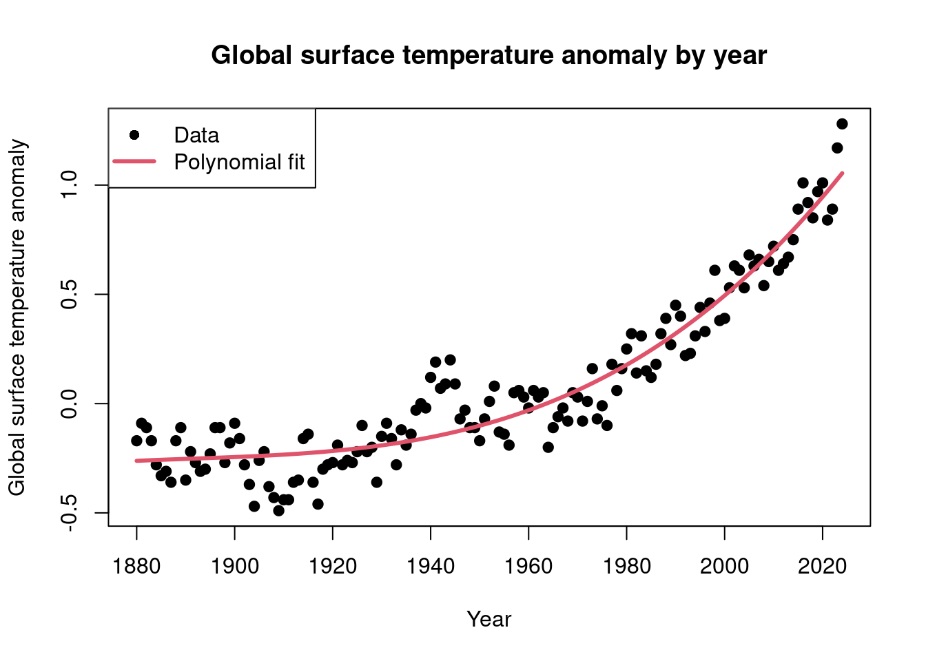
```
Sometimes, the data are plotted as blues and reds
```
image(x = data$year, z = matrix(data$temperature, ncol = 1), 
      col = hcl.colors(11, 'Blue-Red 3'), xlab = 'Year', ylab = '',
      main = 'Color-based global surface temperature anomaly by year')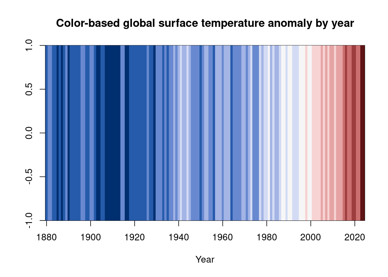
```
as in the plot above.)